21. Multiple Integrals in Curvilinear Coordinates
a. Integrating in Polar Coordinates
5. Converting & Mixing, Rectangular & Polar Coordinates
Sometimes it is useful to use polar coordinates instead of rectangular coordinates when computing an integral. Other times it is best to use rectangular coordinates for one part of an integral and polar coordinates for another part in the same problem.
Converting Rectangular to Polar Coordinates
Sometimes the antiderivative of the integrand is not known, making the integral difficult if not impossible. By converting to polar coordinates, we can simplify the integral greatly.
Compute the integral \(\displaystyle I =\int_0^{3/\sqrt{2}}\int_y^{\sqrt{9-y^2}} \cos(x^2+y^2)\,dx\,dy\)
This integral is very hard to do in rectangular coordinates, since we do not know the antiderivative of \(\cos(x^2+y^2)\). However, converting to polar coordinates drastically simplifies the problem. First, we plot the region. From the integral, we see that the region of integration is \(y \le x \le \sqrt{9-y^2}\). The left and right curves intersect when \[ y=\sqrt{9-y^2} \quad \Rightarrow \quad 2y^2=9 \quad \Rightarrow \quad y=\pm\dfrac{3}{\sqrt{2}} \]
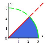
The upper limit for \(y\) is \(\dfrac{3}{\sqrt{2}}\) which is precisely
the intersection point and the lower limit is \(y=0\) as shown in the plot.
We now convert to polar coordinates. Substituting \(x^2+y^2=r^2\), the
integrand becomes \(\cos(r^2)\). From the plot, we see the
bounds on \(r\) and \(\theta\) are:
\[
0 \le r \le 3 \qquad
0 \le \theta \le \dfrac{\pi}{4}
\]
Remember that the differentials become \(dA=dx\,dy=r\,dr\,d\theta\) so that
the polar integral is computed as
\[\begin{aligned}
I&=\int_0^{\pi/4}\int_0^3\cos(r^2) r\,dr\,d\theta
=\int_0^{\pi/4}\,d\theta\int_0^3 r\,\cos(r^2)\,dr \\
&=\dfrac{\pi}{4} \left[\dfrac{1}{2}\sin(r^2)\right]_0^3
=\dfrac{\pi}{8} \sin(9)
\end{aligned}\]
In the following example, algebraic manipulation as well as polar coordinates are used to solve the problem.
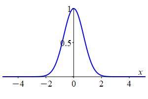
Compute the improper integral \(\displaystyle I=\int_{-\infty}^\infty e^{-x^2}\,dx =\lim_{R\to\infty}\int_{-R}^R e^{-x^2}\,dx\) by using polar coordinates
First, we plot the integrand to observe the shape of the function. Notice how the function asymptotically approaches \(0\) in the limit as \(x\rightarrow\pm\,\infty\). This property will allow us to compute the improper integral.
We start by manipulating the integral algebraically. We first square \(I\), letting the dummy variable in the second \(I\) become \(y\), so that we don't confuse the two differentials: \[\begin{aligned} I^2&=\lim_{R\to\infty}\int_{-R}^R e^{-x^2}\,dx\int_{-R}^R e^{-y^2}\,dy \\ &=\lim_{R\to\infty}\int_{-R}^R\int_{-R}^R e^{-x^2-y^2}\,dx\,dy \end{aligned}\] From here, we switch to polar coordinates by substituting \(x^2+y^2=r^2\) and \(dx\,dy=r\,dr\,d\theta\) in the integral. The integration is performed over the entire \(xy\) plane, so the bounds on \(r\) and \(\theta\) become \[ 0 \le r \le \infty \qquad 0 \le \theta \le 2\pi \] So \(I^2\) in polar coordinates is \[\begin{aligned} I^2&=\lim_{R\to\infty}\int_0^{2\pi}\int_0^R e^{-r^2}r\,dr\,d\theta \\ &=\int_0^{2\pi} \,d\theta\lim_{R\to\infty}\int_0^R e^{-r^2}r\,dr =2\pi\lim_{R\to\infty}\left[-\,\dfrac{1}{2}e^{-r^2}\right]_0^R \\ &=-\pi\lim_{R\to\infty}\left[e^{-r^2}\right]_0^R =-\pi\left[\lim_{R\to\infty}e^{-R^2}-1\right] =\pi \end{aligned}\] Thus, taking the square root, \[ I=\sqrt{\pi} \]
This result is essential in statistics, where the function \(p(x)=\dfrac{1}{\sqrt{\pi}}e^{-x^2}\) is called the Gaussian or normal probability density function, which gives the probability density that a continuous random variable takes on the value \(x\). In particular, if you have an interval \([a,b]\), then the integral \(\displaystyle \int_a^b p(x)\,dx\), gives the probability that the random variable lies within the interval. The function \(e^{-x^2}\) is divided by \(I=\sqrt{\pi}\) so that the total probability equals \(1\), i.e. \(\displaystyle \int_{-\infty}^\infty p(x)\,dx=1\).
Compute \(\displaystyle \iint e^{\sqrt{x^2+y^2}}\,dx\,dy\) over the region between the circles \(x^2+y^2=4\) and \(x^2+y^2=9\).
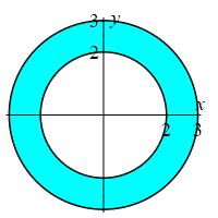
\(I = 2e^2\pi(2e-1) \approx 205.975\)
We start by converting the integral into polar coordinates by substituting \(x^2 + y^2 = r^2\) and \(dx\,dy = r\,dr\,d\theta\). Note that the two bounding circles become \(r^2 = 4\) and \(r^2 = 9\), so the bounds on \(r\) and \(\theta\) become \[ 2 \le r \le 3 \quad \text{and} \quad 0 \le \theta \le 2\pi \] The integral is now \[\begin{aligned} I = \int_0^{2\pi} \int_2^3 e^r\,r\,dr\,d\theta = 2\pi \int_2^3 r\,e^r\,dr \end{aligned}\] We solve this using integration by parts. Let \[\begin{aligned} u &= r &dv &= e^r\,dr \\ du&=dr \quad &v &= e^r \end{aligned}\] Now we have \[\begin{aligned} I &= 2\pi\left[r\,e^r-\int e^r\,dr\right]_2^3 = 2\pi\left[\rule{0pt}{10pt}r\,e^r-e^r\right]_2^3 \\ &= 2\pi(3e^3-e^3-2e^2+e^2) \\ &= 2e^2\pi(2e-1) \approx 205.975 \end{aligned}\]
mj
Mixing Rectangular and Polar Coordinates
Sometimes it is useful to use polar coordinates on part of the integral and rectangular coordinates on another part, as in the example below.
Compute the integral \(\displaystyle \iint xy\,dA\) between the line \(y=3-x\) and the quarter circle \(y=\sqrt{9-x^2}\).
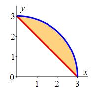
This integral can be computed using either rectangular or polar coordinates. However, it is easier to compute the integral over a quarter circle in polar coordinates and subtract the integral over a triangle. Mathematically, we express this as: \[ \iint_R xy\,dA=\iint_\text{quarter circle}xy\,dA-\iint_\text{triangle}xy\,dA \] First, we use polar coordinates to integrate of \(f=xy\) inside the quarter circle \(y=\sqrt{9-x^2}\) in the first quadrant: \[\begin{aligned} &\iint_\text{quarter circle} xy\,dA =\iint (r\cos\theta)(r\sin\theta)\,r\,dr\,d\theta \\ &=\int_0^{\pi/2}\int_0^3 r^3\sin\theta\cos\theta\,dr\,d\theta =\int_0^3 r^3\,dr\int_0^{\pi/2}\sin\theta\cos\theta\,d\theta \\ &=\left[\dfrac{1}{4}r^4\right]_{r=0}^3 \left[\dfrac{\sin^2\theta}{2}\right]_0^{\pi/2} =\dfrac{3^4}{4}\left(\dfrac{1}{2}-0\right) =\dfrac{81}{8} \end{aligned}\] Next, we use rectangular coordinates to integrate the function \(f=xy\) under the line \(y=3-x\) from \(x=0\) to \(x=3\) \[\begin{aligned} &\iint_\text{triangle}xy\,dA =\int_0^3\int_0^{3-x} xy\,dy\,dx =\int_0^3 \left[x\dfrac{y^2}{2}\right]_{y=0}^{3-x}\,dx \\ &=\dfrac{1}{2} \int_0^3 x(3-x)^2\,dx =\dfrac{1}{2}\int_0^3 (9x-6x^2+x^3)\,dx \\ &=\dfrac{1}{2}\left[\dfrac{9}{2}x^2-2x^3+\dfrac{1}{4}x^4\right]_0^3 =\dfrac{1}{2}\left(\dfrac{9}{2}(3)^2-2(3)^3+\dfrac{1}{4}(3)^4\right) =\dfrac{27}{8} \end{aligned}\] Thus, the net integral is \[\begin{aligned} \iint xy\,dA &=\iint_\text{quarter circle}xy\,dA-\iint_\text{triangle}xy\,dA \\ &=\dfrac{81}{8}-\,\dfrac{27}{8} =\dfrac{27}{4} \end{aligned}\]
A quarter circle \(x^2+y^2\le 1\) is cut out of the square \(0\le x\le1\) by \(0\le y\le1\) made from plastic with density \(\delta=x^2+y^2\). Find the mass of the piece of plastic outside the quarter circle.
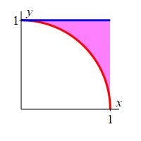
Find the mass of the square and subtract the mass of the quarter circle.
\(M = \dfrac{2}{3} - \dfrac{\pi}{8} \approx .274\)
Using rectangular coordinates, the mass of the square is: \[\begin{aligned} M_{\text{square}} &= \int_0^1 \int_0^1 x^2+y^2 \,dx\,dy \\ &= \int_0^1 x^2\,dx \int_0^1 dy + \int_0^1 dx \int_0^1 y^2\,dy \\ &= \left[\dfrac{1}{3}x^3\right]_{x=0}^{x=1} \left[\rule{0pt}{10pt}y\right]_{y=0}^{y=1} + \left[\rule{0pt}{10pt}x\right]_{x=0}^{x=1} \left[\dfrac{1}{3}y^3\right]_0^1 \\ &= \dfrac{1}{3}\cdot1 + 1\cdot\dfrac{1}{3} = \dfrac{2}{3} \end{aligned}\] Using polar coordinates, the mass of the quarter circle is: \[\begin{aligned} M_{\text{quarter circle}} &= \int_0^{\pi/2} \int_0^1 r^2\cdot r\,dr\,d\theta = \dfrac{\pi}{2} \int_0^1 r^3\,dr \\ &= \dfrac{\pi}{2} \left[\dfrac{1}{4}r^4\right]_0^1 = \dfrac{\pi}{8} \end{aligned}\] Thus the mass of the piece outside the quarter circle is \[ M = M_{\text{square}} - M_{\text{quarter circle}} = \dfrac{2}{3} - \dfrac{\pi}{8} \approx .274 \]
mj
Heading
Placeholder text: Lorem ipsum Lorem ipsum Lorem ipsum Lorem ipsum Lorem ipsum Lorem ipsum Lorem ipsum Lorem ipsum Lorem ipsum Lorem ipsum Lorem ipsum Lorem ipsum Lorem ipsum Lorem ipsum Lorem ipsum Lorem ipsum Lorem ipsum Lorem ipsum Lorem ipsum Lorem ipsum Lorem ipsum Lorem ipsum Lorem ipsum Lorem ipsum Lorem ipsum